Fecal Coliform Concentrations in the Upper Cohansey River Watershed Predicted by Air Temperature, Discharge, and Land Use

Introduction

Preventing water pollution and improving environmental water quality are topics of importance for Extension education nationwide. These topics have relevance for diverse clientele, and they require cross-disciplinary understanding and applied research (Vaughn, 1989), making them ideal targets to benefit from Extension expertise.

In the United States, fecal pathogens are listed as the number one pollutant for rivers, as well as being the third most prevalent pollutant for bays and estuaries, second for coastlines, and third for wetlands (U.S. Environmental Protection Agency, 2014). Indicators of these pathogens include fecal coliform, enterococcus, and Escherichia coli. Understanding the physical factors that influence water pollutant concentrations is important in the education of clientele groups such as watershed associations and nongovernmental organizations that seek appropriate mitigation actions.

The Upper Cohansey River Watershed is located in southwestern New Jersey in a predominantly agricultural area close to Delaware Bay (Figure 1). Located at its downstream end is Sunset Lake, which is of local importance for supporting a swimming beach available to residents of the City of Bridgeton. This beach is closed regularly during the summer due to fecal coliform bacteria (FC) concentration levels that exceed the standard for primary contact recreation (New Jersey Administrative Code, 2011). This situation is not unusual in New Jersey, where 41% of watersheds did not meet their designated recreational uses due to bacteria concentrations in 2008 (New Jersey Department of Environmental Protection [NJDEP], 2009).

Figure 1.
Location of the Upper Cohansey River Watershed

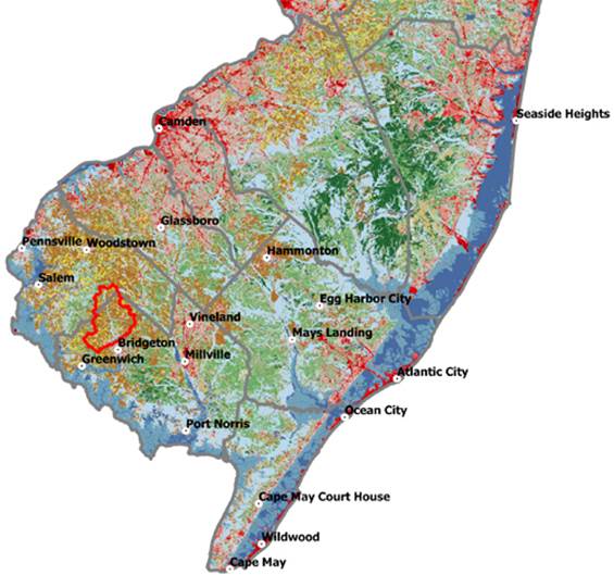
The watershed, located near Bridgeton, New Jersey, is outlined in red. Color coding indicates land use: Red and pink are urban or suburban development; greens are forest; and brown and yellow are crops and pasture (Multi-Resolution Land Characteristic Consortium, 2014a).

In 2003, a total maximum daily load was proposed for FC for the uppermost part of the Upper Cohansey River Watershed, with potential sources including agriculture, livestock, wildlife, and septic systems (NJDEP, 2003). In 2009, Rutgers Cooperative Extension Water Resources Program released a data report finding exceedances in FC levels throughout this uppermost part of the watershed, with 36% of samples exceeding the nominal benchmark of 200 colony-forming units (CFU)/100 ml. Microbial source tracking indicated the presence of human fecal bacteria in some subwatersheds (Rutgers Cooperative Extension Water Resources Program, 2009).

After the 2009 report, New Jersey Department of Environmental Protection and Cumberland County Department of Health undertook actions to remove potential sources of human contamination. Also during that time, the City of Bridgeton undertook actions to reduce the impact of wildlife on Sunset Lake water quality.

The objectives of the study reported in this article were (a) to determine whether actions in the watershed had eliminated or reduced human or nonhuman animal sources of fecal contamination; and (b) to investigate whether environmental variables were associated with fecal contamination.

Methods

Historical Data for Sunset Lake Beach 2002–2011

Results from Cumberland County Department of Health routine sampling of the swimming beach at Sunset Lake from 2002 through 2011 were compiled. Samples exceeding a nominal benchmark of 200 CFU/100 ml for FC were tabulated, and likelihood ratio tests were used to determine whether there were differences in the proportion of exceedances across months or across years. If multiple samples were taken on the same day, values for those samples were averaged, and a single value was used.

FC Concentrations in the Cohansey River and Tributaries

Grab samples of water were collected from the Cohansey River and tributaries and analyzed for FC by a commercial laboratory (Environmental Protection Agency standard method SM 9221/9222 series by membrane filtration, Q.C. Laboratories, Vineland, NJ). Seventy-five samples were collected across 14 locations in the Upper Cohansey River Watershed from February 2012 through October 2013 in an observational, unbalanced experiment. To determine the source of FC, samples from June, July, and August 2013 were sent to a commercial laboratory for microbial source tracking. The test used genetic analysis of a specific bacteria, Bacteroides, to determine whether the bacteria in the samples were from human or nonhuman sources (quantitative polymerase chain reaction, EMSL Analytical, Cinnaminson, NJ).

Geographic Analyses

The area of each sampled subwatershed was determined through the use of GRASS GIS routines r.watershed and r.water.outlet (GRASS GIS Development Team, 2014) within the QGIS software package (QGIS Development Team, 2014). Proportions of land uses within each of these areas were determined by using the National Land Cover Database 2011 (Multi-Resolution Land Characteristic Consortium, 2014b). A similar procedure was followed for land uses in a 90-m (300-ft) buffer around streams in each sampled subwatershed. Other geographic data were obtained from New Jersey Department of Environmental Protection (NJDEP, 2014).

Weather and Stream Flow Data

Mean air temperature and precipitation data were obtained from New Jersey Weather and Climate Network for a station in Upper Deerfield, NJ, approximately 5.5 km (3.4 mi) from the center of the watershed (New Jersey Weather and Climate Network, 2014). Discharge for the main stem of the Cohansey River was obtained for U.S. Geological Survey station 01412800, located approximately in the center of the watershed (U.S. Geological Survey, 2014).

Statistical Analyses

For 11% of samples, FC concentration was greater than 600 CFU/100 ml and was recorded as 600 CFU/100 ml.

A mixed effects model was generated. It related FC concentration to sample location, month of collection, and year of collection, with year treated as a random variable (Pinheiro & Bates, 2000). Means across levels of these factors were separated with Tukey-adjusted least-square means.

To identify factors that may affect FC concentration, Spearman correlations between FC concentration and measured environmental variables were explored. Spearman correlations do not rely on the assumptions that data are normally distributed or linearly related. Temporal variables were 3-day and 5-day antecedent air temperatures, 3-day and 5-day antecedent precipitation levels, water temperature, and discharge in the main stem of the river. Spatial variables related to sample location were the drainage area of the subwatershed, proportions of major land uses in the subwatershed, and proportions of major land uses in 90-m (300-ft) stream buffers. Land uses were highly correlated across subwatersheds. Therefore, a land use index was created, using principal components analysis, to capture the variability in major land uses: agriculture, development, forest, and wetland. A similar procedure was followed for land uses in the 90-m (300-ft) stream buffers.

A final fixed effects model was developed. It related FC concentration to significant environmental variables: 3-day antecedent air temperature, river discharge, and land use index within the 90-m (300-ft) stream buffers. These variables were selected on the basis of their marginal statistical significance when added to the model and improvement of model Akaike information criterion. This method minimized the inclusion of co-correlated terms. Model residuals were checked for normality and homogeneity.

Statistical analyses were conducted by using R (R Core Team, 2014), including packages nmle for mixed models, lsmeans for least-square means and multiple comparisons, psych for principal components analysis, Deducer for likelihood ratio tests, and ggplot2 for some plots.

Results

Historical Data for Sunset Lake Beach 2002–2011

From 2002 through 2011, for samples taken from May through August, the proportion of samples exceeding the nominal benchmark for FC concentration of 200 CFU/100 ml was 0.32 (Table 1). Likelihood ratio tests indicated that there were no differences in proportions among months (p = 0.50) but that there were differences among years (p < 0.0001), with portions of exceedances among years ranging from 0.00 to 0.71 (data not shown).

Table 1.
Proportions of Water Samples with Exceedances of the FC Benchmark for the Swimming Beach at Sunset Lake, 2002–2011

Month	Number of samples	Proportion of exceedances
May	8	0.25
June	35	0.23
July	48	0.38
August	35	0.34
May–August	126	0.32

Geographic Analyses

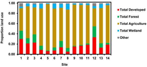
Sampled subwatersheds ranged in size from 3.39 to 118 sq km (1.31–45.5 sq mi). The proportion of agricultural land use ranged from 0.35 to 0.90, with some subwatersheds having significant portions of developed, forested, or wetland lands (Table 2, Figure 2).

Table 2.
Summary Statistics for Proportions of Land Uses Across Sampled Subwatersheds in the Upper Cohansey River Watershed

Land use	Minimum	Median	Maximum
Total agriculture	0.35	0.73	0.90
Total developed	0.05	0.15	0.33
Total forest	0.01	0.08	0.21
Total wetland	0.01	0.06	0.11
Other	0.00	0.01	0.07

Figure 2.
Proportions of Land Uses in Sampled Subwatersheds in the Upper Cohansey River Watershed

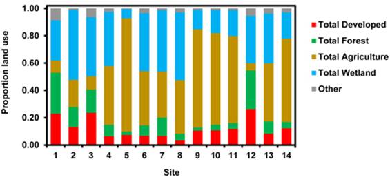
Land use in 90-m (300-ft) stream buffers varied across sampled subwatersheds and generally contained higher proportions of forest and wetland than subwatersheds as a whole (Table 3, Figure 3).

Table 3.
Summary Statistics for Proportions of Land Uses Across 90-m (300-ft) Stream Buffers in Sampled Subwatersheds in the Upper Cohansey River Watershed

Land use	Minimum	Median	Maximum
Total agriculture	0.05	0.40	0.83
Total developed	0.03	0.11	0.26
Total forest	0.02	0.08	0.30
Total wetland	0.07	0.36	0.51
Other	0.01	0.03	0.09

Figure 3.
Proportions of Land Uses in 90-m (300-ft) Stream Buffers in Sampled Subwatersheds in the Upper Cohansey River Watershed

FC Concentrations in the Cohansey River and Tributaries

The proportion of samples collected in 2012–2013 exceeding a nominal benchmark of 200 CFU/100 ml was 0.44 (data not shown). This proportion was somewhat greater than the proportion of exceedances from Rutgers Cooperative Extension Water Resources Program (2009)—0.36; it also was greater than the 0.32 of samples from the swimming beach from 2002–2011 (Table 1). FC concentration exceeding the nominal benchmark was found in most subwatersheds for at least some sample events.

A significant model was found. It related FC concentration to month, site, and year of sampling (p < 0.0001, Nagelkerke pseudo r-square = 0.66), with significant effects for month (p < 0.0001, Figure 4) and sample site (p = 0.048, Figure 5). The effect of year was not significant (p = 0.34). There was a clear seasonal effect, with the greatest FC least-square mean concentration occurring in August and lower concentrations occurring in spring and fall (Figure 4). Least-square means across sites varied less, with some significant differences among sites (Figure 5).

Figure 4.
Least-Square Means of FC Concentration in the Cohansey River and Tributaries Across Months

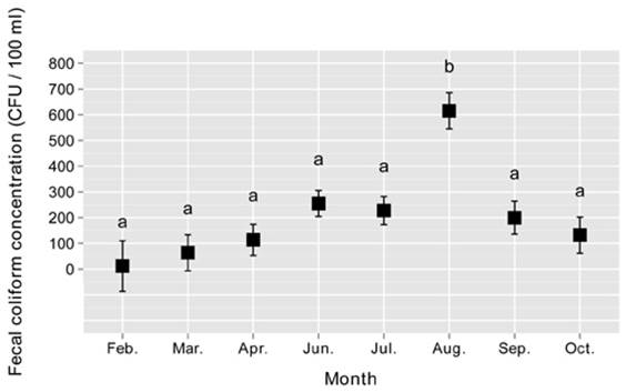
Error bars indicate standard errors of the mean from the analysis. Means with the same letter are not significantly different (alpha = 0.05, Tukey-adjusted comparisons).

Figure 5.
Least-Square Means of FC Concentration in the Cohansey River and Tributaries Across Sample Location

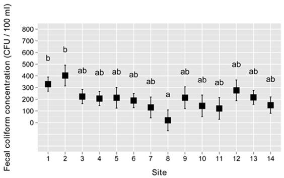
Error bars indicate standard errors of the mean from the analysis. Means sharing a letter are not significantly different (alpha = 0.05, Tukey-adjusted comparisons).

Environmental variables that were significantly correlated with FC concentration were air temperature, 3-day antecedent precipitation, and land use in 90-m (300-ft) stream buffers (Table 4). These variables were used to build a model predicting FC concentration, except that river discharge replaced 3-day antecedent precipitation because the latter failed to be significant in the combined model (Table 5).

Table 4.
Spearman's Rank Correlations Between FC Concentration and Environmental Variables

Environmental variable	Range (metric)	Range (U.S.)	p-value	Spearman's rho
Air temp., 3-day antecedent	4–29°C	39–84°F	< 0.0001	0.48
Air temp., 5-day antecedent	6–28°C	43–83°F	< 0.0001	0.48
Precipitation, 3-day antecedent	0–4.1 cm	0–1.6 in	0.003	0.34
Precipitation, 5-day antecedent	0–7.4 cm	0–2.9 in	ns
Water temp.	12–28°C	53–82°F	ns
Discharge	0.71–3.3 (cu m/s)	25–117 (cu ft/s)	ns
Drainage area	3.4–118 sq km	1.3–45 sq mi	ns
Land use in subwatersheds, principal component 1			ns
Land use in 90-m (300-ft) stream buffers, principal component 1			0.008	0.30

Table 5.
Coefficients and Analysis of Variance for the Model Predicting FC Concentration from Environmental Variables (p < 0.0001, Nagelkerke pseudo r-square = 0.52)

Effect	Coeff. (metric)	Units (metric)	Coeff. (U.S.)	Units (U.S.)	p-value	Marginal Nagelkerke pseudo r-square
Intercept	−139	CFU	−327	CFU	0.0004	0.09
Air temp., 3-day antecedent	10.6	CFU/°C	5.89	CFU/°F	< 0.0001	0.14
Discharge	173	CFU/(cu m/s)	4.89	CFU/(cu ft/s)	< 0.0001	0.25
Land use in 90-m (300-ft) buffers, principal component 1	45.1	CFU/unit	45.1	CFU/unit	0.06	0.02

Microbial Source Tracking

Microbial source tracking detected no human fecal contamination in any samples.

Discussion and Conclusions

The elimination of fecal contamination from human sources following research results published in 2009 suggests that actions by state and county regulators were effective in addressing sources of poor sanitation in the watershed.

Because this was an observational study, causal relationships between FC concentration and environmental factors could not be determined definitively. However, the final model suggested that FC concentration for this watershed is greater in summer months, when there is higher stream discharge, or in locations with certain uses of land buffering streams.

An increase in FC concentration in summer months might suggest that indicator bacteria are surviving better in warm, low-oxygen water in the summer. Flint (1987) found that E. coli could survive up to 260 days in water in the absence of competing or predatory organisms.

Likewise, an increase in FC concentration with higher stream flows or after recent precipitation may suggest that bacteria are surviving in sediments in the streams (LaLiberte & Grimes, 1982; Perry, 2011) and being stirred up during high flows. A flushing effect may also be responsible for the transport of fresh sources of FC to the streams following rains. Another factor may be the turbidity of water during higher flows, as solar radiation limits survival of fecal bacteria in environmental waters (Brookes et al., 2004).

It was not possible to isolate which land uses are associated with higher FC concentration because land uses in the stream buffers were correlated to one another. For example, because the portion of developed land was strongly negatively correlated with the portion of agricultural land, it is not possible to say whether a certain effect was associated with an increase in developed land or a decrease in agricultural area. However, development, forest, and wetland land uses each had positive statistical loadings in the land use index, whereas agriculture had a negative loading. This result is consistent with the idea that FC in this watershed are associated with, for example, storm water from developed lands in stream buffers or wildlife that frequent forest and forested wetland areas. High levels of FC from developed areas have been reported. For example, Dietz, Clausen, Warner, and Filchak (2002) reported FC concentration greater than 1,000 fecal colony units in runoff from a suburban neighborhood.

These results suggest the importance of several potential future actions:

• Further characterization of locations with high FC concentration may be warranted because there were differences in FC concentration among sample locations that were not fully explained by the investigated variables.
• Further speciation of fecal bacteria through microbial source tracking to determine specific wildlife sources may be helpful in formulating mitigation strategies.
• Adding stream buffers where they are lacking may help decrease FC load and lower stream temperatures. Improving storm water management in developed areas may decrease stream flows and pollutant delivery.

It is hoped that these results and conclusions will be of use for Extension professionals working in water resources and for their clientele in guiding future Extension education and applied research activities.

Acknowledgments

The project described herein was the result of a partnership of the Cohansey Area Watershed Association, the Cumberland County Department of Health, and Rutgers Cooperative Extension.

References

Brookes, J. D., Antenucci, J., Hipsey, M., Burch, M. D., Ashbolt, N. J., & Ferguson, C. (2004). Fate and transport of pathogens in lakes and reservoirs. Environment International, 30, 741–759.

Dietz, M. E., Clausen, J. C., Warner, G. S., & Filchak, K. K. (2002). Impacts of Extension education on improving residential stormwater quality: Monitoring results. Journal of Extension [online], 40(6) Article 6RIB5. Available at: www.joe.org/joe/2002december/rb5.php

Flint, K. P. (1987). The long-term survival of Escherichia coli in river water. Journal of Applied Bacteriology, 63, 261–270.

GRASS GIS Development Team. (2014). GRASS GIS. Retrieved from grass.osgeo.org/

LaLiberte, P., & Grimes, J. (1982). Survival of Escherichia coli in lake bottom sediment. Applied and Environmental Microbiology, 43, 623–628.

Multi-Resolution Land Characteristic Consortium. (2014a). National land cover database 2006 product legend. Retrieved from www.mrlc.gov/nlcd06_leg.php

Multi-Resolution Land Characteristic Consortium. (2014b). National land cover database 2011. Retrieved from www.mrlc.gov/nlcd2011.php

New Jersey Administrative Code. (2011). N.J.A.C. 7:9B surface water quality standards. Retrieved from www.nj.gov/dep/rules/rules/njac7_9b.pdf

New Jersey Department of Environmental Protection. (2003). Total maximum daily loads for fecal coliform to address 27 streams in the Lower Delaware Water Region. Retrieved from www.epa.gov/waters/tmdldocs/NJ-2003-Fecal Coliform-27 Streams Lower Delaware Region.pdf

New Jersey Department of Environmental Protection. (2009). 2008 New Jersey integrated water quality monitoring and assessment report. Retrieved from www.state.nj.us/dep/wms/bwqsa/2008_integrated_report.htm

New Jersey Department of Environmental Protection. (2014). Geographic information systems statewide layers. Retrieved from www.state.nj.us/dep/gis/stateshp.html

New Jersey Weather and Climate Network. (2014). New Jersey Weather and Climate Network data viewer. Retrieved from www.njweather.org/data/daily

Perry, A. (2011). E. coli: Alive and well, probably in a streambed near you. Agricultural Research, July:20. Retrieved from www.ars.usda.gov/is/AR/archive/jul11/ecoli0711.htm.

Pinheiro, J., & Bates, D. (2000). Mixed-effects models in S and S-Plus. New York, NY: Springer-Verlag.

QGIS Development Team. (2014). QGIS. Retrieved from www.qgis.org/

R Core Team. (2014). R: A language and environment for statistical computing. Vienna, Austria: R Foundation for Statistical Computing. Retrieved from www.R-project.org/

Rutgers Cooperative Extension Water Resources Program. (2009). Upper Cohansey River Watershed restoration and protection plan: Data report. Retrieved from www.water.rutgers.edu/Projects/UpperCohansey/Upper_Cohansey_River_Watershed_Data_Report_120409.pdf

U.S. Environmental Protection Agency. (2014). National summary of state information. Water quality assessment and total maximum daily loads information. Retrieved from www.epa.gov/waters/ir/

U.S. Geological Survey. (2014). National Water Information System: Web interface. Retrieved from waterdata.usgs.gov/nj/nwis/uv

Vaughn, G. F. (1989). Water quality as an issue: What does this mean? Journal of Extension [online], 27(4) Article 4FRM1. Available at: www.joe.org/joe/1989winter/f1.php