Cate-Nelson Analysis for Bivariate Data Using R-project

Introduction

In Extension, it is helpful to be able to analyze data in innovative ways, especially if the results can be shown in a simple format that is easily interpretable by clientele.  For example, Gareau, Smith, Barbercheck, and Mortensen (2010) showed how spider plots could be used to display multiple variables describing cover crop value in intuitive and simple plots.  Focusing on innovative analyses, Hollingsworth, Collins, Smith, and Nelson (2011) discussed how rank-sum test could be used to indicate statistical correlation among survey responses, and Santos and Clegg (1999) discussed the use of factor analysis to find response patterns in survey data.

Cate-Nelson Analysis

Cate–Nelson analysis is a technique traditionally used in agronomy, particularly to calibrate soil test data to an expected crop response. The idea behind the analysis is to divide the data into two groups:  those data where a change in the x variable is likely to correspond to a response in the y variable and those data where a change in x is unlikely to correspond to a change in y.

Following the traditional application, for example, were Heckman and others (2006) who used Cate–Nelson models to determine the soil test phosphorus values above which a corn yield response is unlikely. Somewhat innovative applications include O'Toole and Herbert (2002), who used the analysis to look at the yield of sweet corn versus corn stalk nitrate concentration, and Mangiafico and Guillard (2006), who used the analysis to determine the soil nitrate levels above which a color response in turfgrass was unlikely.

In an application not related to crop response, Mangiafico, Newman, Mochizuki, and Zurawski (2008) used a Cate–Nelson analysis to relate the number of good practices reported in a survey of plant nurseries to the size of those nurseries. This use indicates that the technique could be used for a wide variety of data sets, to divide bivariate data into two populations to illustrate the relationship between the two variables and present that relationship simply and graphically.

• In a Cate–Nelson analysis, the data are divided so that they fall into four quadrants, (Figure 1, indicated with Roman numerals):
• Points in Quadrant IV are data with x values below the critical-x value, and y values below the critical-y value.
• Those in Quadrant II are data with x values above the critical-x and y values above the critical-y.
• The analysis finds the lines that best divide the data to maximize the data falling into Quadrants II and IV.
• Points in Quadrants I and III are data that do not follow the predictive model represented by the points in the other two quadrants.

Figure 1.
Example Plot from a Cate–Nelson Analysis Using the Included Code for R-Project

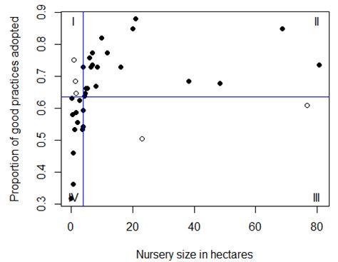
Note:  Example data from Mangiafico, Newman, Mochizuki, & Zurawski (2008). Blue lines indicate critical-x value and critical-y value separating the data into four quadrants. Roman numerals designate quadrants of the plot. Data that fall into quadrants II and IV are in accordance with the model (smaller nurseries with lower scores and larger nurseries with higher scores) and are indicated by solid points. Data that fall into quadrants I and III are errors in prediction by the model and are indicated by open points.

Statistical Analysis

Hand Calculation or Spreadsheet

One of the traditional advantages of a Cate–Nelson analysis was that it could be done graphically once the data had been plotted, with no statistical calculations. Cate and Nelson (1971), however, reported a statistical method by which the critical-x could be found by calculating the Sum of Squares values for each potential critical-x value and choosing the one that maximizes the Sum of Squares. Because the procedure requires only relatively simple calculations, it could be performed by hand for small datasets or could be partially automated in a spreadsheet program, such as Excel. However, analyzing large datasets in this manner could prove unwieldy, and repeated calculations could easily introduce errors.

SAS Software

A simple SAS procedure, utilizing PROC ANOVA to calculate automatically the Sum of Squares is presented below (after Kopp & Guillard, 2002). This procedure requires, however, that the potential critical-x value in the third line of the code be changed iteratively to each of the potential critical values for the dataset, and the procedure re-run each time, so that the critical-x value that maximizes the ANOVA SS in the output can be selected. This iterative procedure is likely to be burdensome for large datasets. Furthermore, the critical-y value and error rate would have to be determined manually afterwards. There is the potential to automate this procedure further, however, to accomplish these tasks.

R-Project for Statistical Computing

A procedure to complete a Cate–Nelson analysis automatically in R-project (see Mangiafico, 2013) was written and is presented below. The code can be copied and pasted into the R-project command line to run the analysis, produce the relevant plots, and display the resultant statistics. Users can simply change the x and y values in the beginning of the program to reflect their own data.

The output contains the relevant statistics, in blue, indicating the number of observations, critical-x value, critical-y value, and the number and percentage of observations falling into each quadrant:

[1] "n"
[1] 38
[1] "Critical x"
[1] 4.035
[1] "Critical y"
[1] 0.6355
[1] "Quadrant I"
[1] 3
[1] 0.07894737
[1] "Quadrant II"
[1] 20
[1] 0.5263158
[1] "Quadrant III"
[1] 2
[1] 0.05263158
[1] "Quadrant IV"
[1] 13
[1] 0.3421053
[1] "Quadrants I + III"
[1] 5
[1] 0.1315789

The plots include a plot of the data and blue lines indicating the critical-x and critical-y values (Figure 1).

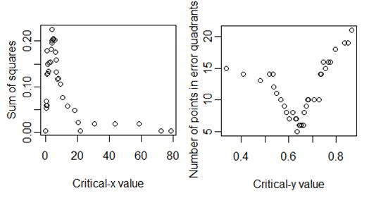
Additional plots show the relationship between the Sum of Squares and the potential critical-x values, and between the number of points that fall into the error quadrants and the critical-y values (Figure 2). These are useful to understand, for example, the range of critical values over which the Sum of Squares is relatively maximized.

Figure 2.
Plots Indicating the Critical-x Value That Maximizes Sum of Squares and the Critical-y Value That Minimizes Errors

The code also produces a Chi-square test as a post-hoc test. This is not a necessary statistic, but can be used to emphasize that a relationship exists between the variables when divided into groups according to the Cate–Nelson procedure.

Pearson's Chi-squared test with Yates' continuity correction

data:  data.frame(row.1, row.2)
X-squared = 17.2806, df = 1, p-value = 3.225e-05

Conclusion

Cate-Nelson analysis can act as another tool for Extension researchers to analyze data and present it in a simple format. Dividing the data into two populations with this analysis is useful to tease out a relationship in bivariate data when other types of analyses may fail. Using the included R-project code allows the user to perform the analysis without an extensive investment in calculations by hand or spreadsheet.

References

Cate, R. B., & Nelson, L.A. (1971). A simple statistical procedure for partitioning soil test correlation data into two classes. Soil Science Society of America Proceedings 35, 658–660.

Gareau, T. P., Smith, R. G., Barbercheck, M. E., & Mortensen, D. A. Spider plots: A tool for participatory extension learning. Journal of Extension [On-line], 48(5) Article 5TOT8. Available at: http://www.joe.org/joe/2010october/tt8.php

Heckman, J. R., Jokela, W., Morris, T., Beegle, D. B., Sims, J. T., Coale, F. J., Herbert, S., Griffin, T., Hoskins, B., Jemison, J., Sullivan, W. M., Bhumbla, D., Estes, G., & Reid, W .S. (2006). Soil test calibration for predicting corn response to phosphorus in the Northeast USA. Agronomy Journal 98, 280–288.

Hollingsworth, R. G., Collins, T. P., Smith, V. E., & Nelson, S. C. (2011). Simple statistics for correlating survey responses. Journal of Extension [On-line], 49 (5) Article 5TOT7. Available at: http://www.joe.org/joe/2011october/tt7.php

Kopp, K. L, & Guillard, K. (2002). Relationship of turfgrass growth and quality to soil nitrate desorbed from anion exchange membranes. Crop Science 42,1232–1240.

 Mangiafico, S.S . (2013). Using R-project for free statistical analysis in Extension research. Journal of Extension [On-line], 51(3) Article 3TOT3. Available at: http://www.joe.org/joe/2013june/tt3.php

Mangiafico, S. S.. & Guillard, K. (2006). Anion exchange membrane soil nitrate predicts turfgrass color and yield. Crop Science 46, 569–577.

Mangiafico, S. S., Newman, J. P., Mochizuki, M. J., & Zurawski, D. (2008). Adoption of sustainable practices to protect and conserve water resources in container nurseries with greenhouse facilities. Acta Horticulturae 797, 367–372.

O'Toole, B. M., & Herbert, S. J. (2002). Nitrogen sufficiency stalk test for sweet corn.

University of Massachusetts Cooperative Extension. Amherst, MA. Retrieved from: http://extension.umass.edu/cdle/sites/extension.umass.edu.cdle/files/research/2002-03-nitrogen-sufficiency-stalk-test-for-sweet-corn.pdf.

Santos, J. R. A., & Clegg, M. D. (1999) Factor analysis adds new dimension to Extension surveys. Journal of Extension [On-line], 37(5) Article 5RIB6. Available at: http://www.joe.org/joe/1999october/rb6.php

SAS Code

DATA dataset;
INPUT x y;
 IF x < 4.035 THEN GROUP=1; ELSE GROUP=2;

 *** Note: The 4.035 value above must be changed manually
           to test each potential critical-x value,
           and the procedure re-run until the critical-x
           that maximizes Anova SS in the output is found.
           Potential critical-x are determined by ordering
           the data by x value, and choosing each x value
           midway between each adjacent pair of data points.
           ;
***  Data from Mangiafico, S.S., Newman, J.P., Mochizuki, M.J.,
           & Zurawski, D. (2008). Adoption of sustainable
           practices to protect and conserve water resources in
           container nurseries with greenhouse facilities.
           Acta horticulturae 797, 367–372.
           ;
CARDS;
   68.55    0.85
    6.45   0.729
    6.98   0.737
    1.05   0.752
    4.44   0.639
    0.46   0.579
    4.02   0.594
    1.21   0.534
    4.03   0.541
    6.05   0.759
   48.39   0.677
    9.88    0.82
    3.63   0.534
   38.31   0.684
   22.98   0.504
    5.24   0.662
    2.82   0.624
    1.61   0.647
   76.61   0.609
    4.64   0.647
    0.28   0.632
    0.37   0.632
    0.81   0.459
    1.41   0.684
    0.81   0.361
    2.02   0.556
   20.16    0.85
    4.04   0.729
    8.47   0.729
    8.06   0.669
   20.97    0.88
   11.69   0.774
   16.13   0.729
    6.85   0.774
    4.84   0.662
   80.65   0.737
    1.61   0.586
     0.1   0.316
;
PROC ANOVA;
 CLASS GROUP;
MODEL Y=GROUP;

RUN;
QUIT;

R-project Code

##--------------------------------------------------------------------
## Cate-Nelson analysis
## Code written by Salvatore Mangiafico, Rutgers Cooperative Extension
##  mangiafico@njaes.rutgers.edu
## Data from Mangiafico, S.S., Newman, J.P., Mochizuki, M.J.,
##   & Zurawski, D. (2008). Adoption of sustainable practices
##   to protect and conserve water resources in container nurseries
##   with greenhouse facilities. Acta horticulturae 797, 367–372.
## Notes:
##  One known issue: The program will produce errors if the two lowest
## or highest x values are equal.
##-------------------------------------------------------------------

##----------------------------------------------------------
##---------- input x and y data-----------------------------
x <-  c(68.55,6.45,6.98,1.05,4.44,0.46,4.02,1.21,4.03,
  6.05,48.39,9.88,3.63,38.31,22.98,5.24,2.82,1.61,
  76.61,4.64,0.28,0.37,0.81,1.41,0.81,2.02,20.16,
  4.04,8.47,8.06,20.97,11.69,16.13,6.85,4.84,80.65,1.61,0.10)
y <-  c(0.850,0.729,0.737,0.752,0.639,0.579,0.594,0.534,
  0.541,0.759,0.677,0.820,0.534,0.684,0.504,0.662,
  0.624,0.647,0.609,0.647,0.632,0.632,0.459,0.684,
  0.361,0.556,0.850,0.729,0.729,0.669,0.880,0.774,
  0.729,0.774,0.662,0.737,0.586,0.316)
##----------------------------------------------------------

##----------------------------------------------------------
##-----order by x and create clx variable for calculation---
n <- length(x)
xgroup <- c('a','b')
ygroup <- c('c','d')
for (i in c(2:n))
  { xgroup[i] <-  c('b')
  ygroup[i] <-  c('d') }
dataset <- data.frame(x = x, y = y, xgroup = as.factor(xgroup),
  ygroup = as.factor(ygroup))
dataset$ObsNo <- 1:n
dataset <- dataset[with(dataset, order(x, y)), ]
dataset$clx[1] <- 0
for(k in c(2:n))
  {dataset$clx[k] <- (dataset$x[k] + dataset$x[k-1])/2}
dataset$clx[1] <- min(dataset$clx[2:n])
plot(dataset$x,dataset$y, pch=16,
  xlab="Nursery size in hectares",
  ylab="Proportion of good practices adopted")
##--------------------------------------------------------

##--------------------------------------------------------
## ------ determine final critical x, and reset x-groupings ------
m <- n-2
dataset$SS[1] <- 0
for(j in c(3:m))
  {for (i in c(1:n))
     {dataset$xgroup[i] <- if(dataset$x[i] < dataset$clx[j])
        'a' else 'b'}
        fit <- lm(y ~ xgroup, data=dataset)
        fit1 <- anova(fit)
        dataset$SS[j] <- (fit1[1,2])}
dataset$SS[1] <- min(dataset$SS[3:(n-2)])
dataset$SS[2] <- min(dataset$SS[3:(n-2)])
dataset$SS[n-1] <- min(dataset$SS[3:(n-2)])
dataset$SS[n] <- min(dataset$SS[3:(n-2)])
max.ss <- max(dataset$SS)
dataset2 <- subset(dataset, SS == max.ss)
CLX <- dataset2$clx[1]
for (i in c(1:n))
     {dataset$xgroup[i] <- if(dataset$x[i] < CLX)  'a' else 'b'}
par(ask=TRUE)
plot(SS~clx, data=dataset, xlab="Critical-x value",
     ylab="Sum of squares")
## ----------------------------------------------------------

## ----------------------------------------------------------
##-order by y, add cly variable, and determine final critical-y-
dataset <- dataset[with(dataset, order(y, x)), ]
dataset$cly[1] <- 0
for(k in c(2:n))
    { dataset$cly[k] <- (dataset$y[k]+dataset$y[k-1])/2 }
dataset$cly[1] <- min(dataset$cly[2:n])
for(j in c(1:n))
  { for (i in c(1:n))
   { (dataset$ygroup[i]
    <- if(dataset$y[i] < dataset$cly[j]) 'c' else 'd')}
  for (i in c(1:n))
   { dataset$q.i[i] <- with(dataset, ifelse
      (dataset$xgroup[i]=='a' & dataset$ygroup[i]=='d', 1, 0))
     dataset$q.ii[i] <- with(dataset, ifelse
      (dataset$xgroup[i]=='b' & dataset$ygroup[i]=='d', 1, 0))
     dataset$q.iii[i] <- with(dataset, ifelse
      (dataset$xgroup[i]=='b' & dataset$ygroup[i]=='c', 1, 0))
     dataset$q.iv[i] <- with(dataset, ifelse
      (dataset$xgroup[i]=='a' & dataset$ygroup[i]=='c', 1, 0)) }
     dataset$q.err[j] <- (  sum(dataset$q.i) + sum(dataset$q.iii)) }
min.qerr <- min(dataset$q.err)
dataset3 <- subset(dataset, q.err == min.qerr)
CLY <- dataset3$cly[1]
plot(q.err~cly, data=dataset, xlab="Critical-y value",
     ylab="Number of points in error quadrants")
## --------------------------------------------------------------

## --------------------------------------------------------------
## -------- reset y-grouping for final grouping ---------------
for (i in c(1:n))
  { (dataset$ygroup[i] <- if(dataset$y[i] < CLY) 'c' else 'd')
   dataset$q.i[i] <- with(dataset, ifelse
      (dataset$xgroup[i]=='a' & dataset$ygroup[i]=='d', 1, 0))
   dataset$q.ii[i] <- with(dataset, ifelse
      (dataset$xgroup[i]=='b' & dataset$ygroup[i]=='d', 1, 0))
   dataset$q.iii[i] <- with(dataset, ifelse
      (dataset$xgroup[i]=='b' & dataset$ygroup[i]=='c', 1, 0))
   dataset$q.iv[i] <- with(dataset, ifelse
      (dataset$xgroup[i]=='a' & dataset$ygroup[i]=='c', 1, 0)) }
## -----------------------------------------------------------

## -----------------------------------------------------------
## ---------- print results and perform chi-square -----------
q.I <- sum(dataset$q.i)
q.II <- sum(dataset$q.ii)
q.III <- sum(dataset$q.iii)
q.IV <- sum(dataset$q.iv)
print('n')
print(n)
print('Critical x')
print(CLX)
print('Critical y')
print(CLY)
print('Quadrant I')
print(q.I)
print(q.I/n)
print('Quadrant II')
print(q.II)
print(q.II/n)
print('Quadrant III')
print(q.III)
print(q.III/n)
print('Quadrant IV')
print(q.IV)
print(q.IV/n)
print('Quadrants I + III')
print(q.I + q.III)
print((q.I + q.III)/n)
row.1 <- c(q.I, q.II)
row.2 <- c(q.IV, q.III)
chisq.test(data.frame(row.1,row.2))
## ---------------------------------------------------------

## ---------------------------------------------------------
## --------- final plot and clean up data set --------------
for(i in c(1:n))
    { dataset$pchi[i] <- 16}
      dataset$pchi[(dataset$x<CLX)&(dataset$y<CLY)] <- 16
      dataset$pchi[(dataset$x>CLX)&(dataset$y>CLY)] <- 16
      dataset$pchi[(dataset$x>CLX)&(dataset$y<CLY)] <- 1
      dataset$pchi[(dataset$x<CLX)&(dataset$y>CLY)] <- 1
plot(dataset$x,dataset$y,pch=dataset$pchi,
  xlab="Nursery size in hectares",
  ylab="Proportion of good practices adopted")
abline(v=CLX, col="blue")
abline(h=CLY, col="blue")
max.x <- max(dataset$x)
max.y <- max(dataset$y)
min.x <- min(dataset$x)
min.y <- min(dataset$y)
text (min.x+(max.x-min.x)*0.01, min.y+(max.y-min.y)*0.99,
 labels="I")
text (min.x+(max.x-min.x)*0.99, min.y+(max.y-min.y)*0.99,
 labels="II")
text (min.x+(max.x-min.x)*0.99, min.y+(max.y-min.y)*0.01,
 labels="III")
text (min.x+(max.x-min.x)*0.01, min.y+(max.y-min.y)*0.01,
 labels="IV")
dataset <- dataset[with(dataset, order(ObsNo)), ]
dataset <- subset(dataset, select = -clx)
dataset <- subset(dataset, select = -cly)
dataset <- subset(dataset, select = -SS)
dataset <- subset(dataset, select = -q.err)
dataset <- subset(dataset, select = -ObsNo)
#dataset
## ---------------------- END ------------------------------