June 2013
|
June 2013 // Volume 51 // Number 3 // Tools of the Trade // v51-3tt3


Using R-project for Free Statistical Analysis in Extension Research
Abstract
One option for Extension professionals wishing to use free statistical software is to use online calculators, which are useful for common, simple analyses. A second option is to use a free computing environment capable of performing statistical analyses, like R-project. R-project is free, cross-platform, powerful, and respected, but may be difficult for beginners to learn. Using a graphical user interface allows new users to perform common analyses using pull-down menus and dialog boxes without programming knowledge. An example of an R-project program, performing a linear regression and producing relevant plots and statistics, is included.
Introduction
Considering the high demands and limited resources common in Extension education, there is always interest in free resources to increase productivity, and software is no exception. Donaldson (2010) listed a few free software programs that might help Extension professionals do concept-mapping, online polling, and project plan management. Similarly, having access to free software for statistical analysis is desirable because statistical software is often relatively expensive and some packages require further annual fees. These expenses may be difficult to justify for some Extension professionals who may not need to perform statistical analyses very often. The SAS statistical package is often cited for performing statistical procedures of interest in Extension research (Santos, 1999; Santos & Clegg, 1999; Spears & Wilson, 2010). Free alternatives for statistical analysis include online calculators and the R-project for Statistical Computing software.
Using Free Calculators on Websites
Many simple analyses, such as t-tests or linear regression, can be performed using online calculators for the specific analysis. As examples, the website by Wessa (2012) contains modules for many analyses that are free for non-commercial use, and StatsPages.org (2012) maintains links to a fairly impressive collection of these sites. Table 1 lists a few sites with online calculators. Such sites are useful for doing quick analyses, and though there may be some reluctance to trust a website one is unfamiliar with, many of these analyses are standard enough that calculators from legitimate sources are unlikely to contain errors.
| Source | Website | Analyses | Notes |
| GraphPad | www.graphpad.com/quickcalcs/ | Descriptive statistics, Chi-square, t-test, among others | |
| Wessa | wessa.net | Descriptive statistics, some plots, Chi-square, t-test, ANOVA, logistic regression, some non-parametric analyses, among others | Includes R code for modules |
| StatPages | statpages.org | Various | Provides links to a variety of sites offering statistical analyses |
R-project for Statistical Computing
One free, powerful, and well-respected software package for statistical analysis is the R-project for Statistical Computing, or simply R or R-project (R Development Core Team, 2012). R-project is a computing language and environment, and is based on a free version of the programming language S. It has the ability to manipulate data, perform statistical analyses, and generate high-quality plots. Its abilities can be extended through additional downloadable packages designed for specific analyses. It has gained popularity at universities for its pedagogical value in statistics classes and adaptability for specific analyses in research (Vance, 2009).
Advantages of using R-project include:
- It's free.
- It can be installed for Windows, Macintosh, and Unix-like operating systems.
- It's powerful enough to perform complex analyses, comparable to SAS or SPSS.
- There's lots of help available online, including tutorials, books, blogs, and discussion forums. Textbooks are available for purchase.
- It's well-respected and citable. It is used extensively in some fields, and is used in some university courses.
Disadvantages of using R-project include:
- It may be difficult for beginning users to get started. Even if they have experience in SAS or SPSS, users will find that the language R-project uses is quite different.
Using a Graphic User Interface for Simple Analyses
One method to get around the difficulty of learning the R-project language is to use a Graphic User Interface (GUI) that can import data, perform common analyses, and produce plots. A GUI allows users to perform analyses with pull-down menus and dialog boxes rather than needing to write the code. One popular GUI is R Commander (Fox, 2012). Benefits of this GUI include:
- Users can easily input or import datasets.
- Several standard analyses can be performed without any coding experience. These include Chi-square, t-test, linear regression, general linear models, and ANOVA. Parameter estimates and p-values are included in the output.
- The code of each analysis is displayed, to help users learn the language.
R Commander can be installed on Windows machines from R with the command:
install.packages("Rcmdr", dependencies=TRUE)
For each session, Rcmdr is summoned with the command:
library(Rcmdr)
Statistical Analysis in R-project
Once data are properly imported into R-project, most common analyses require only a few lines of code. Interaction of the analyst is usually necessary, though, for exploratory data analysis or to be sure data fit the assumptions of the analysis. There are numerous documents and websites that give examples in R-project code for common analyses. Two examples of useful texts for beginners are those by Verzani (2002) and Muenchen (2011).
Linear Regression Example with R-project
Code for specific analyses, however, could also be assembled like a program so that less experienced users could run the complete analysis without much intervention or knowledge of R-project language. As an example, code for a linear regression analysis is included here.
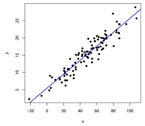
The included code can be simply copied and pasted into the R-project command line prompt or R Commander script window. The code produces a plot of the data with the best-fit line (Figure 1), plots of residuals to check model assumptions, and relevant statistics in blue text:
lm(formula = y ~ x)

Coefficients:
            Estimate Std. Error t value Pr(>|t|)
(Intercept) 5.471087   0.411790   13.29   <2e-16 ***
x           0.201947   0.007503   26.91   <2e-16 ***
---
Signif. codes:  0 '***' 0.001 '**' 0.01 '*' 0.05 '.' 0.1 ' ' 1

Residual standard error: 1.881 on 98 degrees of freedom
Multiple R-squared: 0.8808,     Adjusted R-squared: 0.8796
F-statistic: 724.4 on 1 and 98 DF,  p-value: < 2.2e-16
Users can simply change the x and y values in the beginning of the program to reflect their own data.
Figure 1.
Plot of Hypothetical Data with Best-fit Line Using the Included Code for R-project
Conclusion
Both online calculators and R-project software with a graphical user interface are tools Extension researchers can use to complete simple statistical analyses without a large investment in money or learning the required code. Users are cautioned, though, that statistical analyses should be performed only with an understanding of when they are appropriate and when their underlying assumptions are met.
References
Donaldson, J. L. (2010). Getting acquainted with free software. Journal of Extension [On-line], 48(3) Article 3TOT7. Available at: http://www.joe.org/joe/2010june/tt7.php
Fox, J. (2012). R Commander. Retrieved from: http://cran.r-project.org/web/packages/Rcmdr/index.html
GraphPad Software (2012). QuickCalcs. Retrieved from: http://www.graphpad.com/quickcalcs/
Muenchen, R. A. (2011). R for SAS and SPSS users. New York, NY: Springer.
R Development Core Team. (2012). R: A Language and Environment for Statistical Computing. Vienna, Austria: R Foundation for Statistical Computing. Retrieved August 8, 2012 from http://www.R-project.org.
Santos, J. R. A. (1999). Cronbach's alpha: A tool for assessing the reliability of scales. Journal of Extension [On-line], 37(2) Article 2TOT3. Available at: http://www.joe.org/joe/1999april/tt3.php
Santos, J. R. A., & Clegg, M. D. (1999) Factor analysis adds new dimension to Extension surveys. Journal of Extension [On-line], 37(5) Article 5RIB6. Available at: http://www.joe.org/joe/1999october/rb6.php
Spears, K., & Wilson, M. (2010). "I don't know" and multiple choice analysis of pre- and post-tests. Journal of Extension [On-line], 48(6) Article 6TOT2. Available at: http://www.joe.org/joe/2010december/tt2.php
StatPages.org. (2012). Interactive statistical calculation pages. Retrieved from: http://statpages.org/
Vance, A. (2009). Data Analysts Captivated by R's Power. New York Times, January 7. http://www.nytimes.com/2009/01/07/technology/business-computing/07program.html.
Verzani, J. (2002). SimpleR: Using R for introductory statistics. Retrieved from: http://www.math.csi.cuny.edu/Statistics/R/simpleR
Wessa, P. (2012). Free statistics and forecasting software (calculators). Retrieved from: http://www.wessa.net/
R-project Code
## ---------------------------------------------------------------------------
## --------- linear regression with one independent variable -----------------
## --------- using lm (general linear model) in stats package ----------------
## ---------------------------------------------------------------------------
## ------------------------- input x and y data ------------------------------
## ---------------------------------------------------------------------------
 x <- c(67.54, 24.11, 35.00, 80.42, 15.06, 4.58, 42.20, 45.25, 71.39,
   53.64, 86.96, 46.04, 55.69, 57.93, 20.98, 48.39, 60.08, 34.78, 30.83,
   -21.49, 67.00, 32.32, 84.20, 62.05, 51.85, 54.28, 83.67, 77.09, 42.70,
   71.72, 20.95, 37.67, 57.53, 95.51, 62.77, 61.94, 49.79, 34.58, 64.57,
   6.05, 106.56, 68.40, 32.25, 86.36, 47.75, 56.92, 21.55, 38.50, 79.57,
   47.59, 60.10, 37.71, 66.12, 21.78, 2.82, 3.62, 87.56, 54.23, 44.64,
   25.05, 24.06, 31.11, 46.50, 62.34, 26.12, 49.57, 31.49, 20.61, 27.93,
   -6.62, 42.32, 107.96, 17.85, 67.81, 50.51, 49.06, 28.28, 54.23, 65.17,
   83.77, 60.56, 21.80, 70.17, 22.44, 53.13, 34.06, 10.04, 61.44, 41.05,
   42.75, 87.21, 52.60, 86.87, 65.46, 69.51, 71.78, 26.56, 15.68, 70.33, 71.73)
 y <- c(19.96, 7.73, 15.12, 17.64, 8.48, 5.53, 14.76, 15.84, 17.85,
   16.88, 23.99, 14.85, 17.09, 19.03, 9.00, 14.58, 17.15, 10.91, 12.02,
   2.31, 18.53, 9.30, 24.72, 17.30, 15.91, 13.99, 21.63, 20.89, 15.20,
   19.81, 11.23, 13.98, 19.07, 24.01, 15.35, 13.83, 19.76, 11.53,
   17.50, 8.58, 28.89, 19.25, 8.34, 21.50, 16.03, 19.89, 9.71, 15.61,
   27.03, 11.88, 20.57, 15.09, 16.63, 10.15, 4.83, 9.03, 23.95, 12.94,
   13.20, 10.96, 9.42, 11.91, 15.21, 20.25, 11.04, 14.27, 10.44, 10.51,
   13.94, 3.28, 16.19, 25.66, 7.12, 16.95, 15.29, 16.06, 9.09, 17.84,
   18.73, 22.23, 16.54, 7.75, 21.09, 6.22, 15.67, 12.84, 7.87, 19.56, 12.96,
   16.97, 19.90, 18.94, 21.35, 20.04, 19.76, 20.12, 10.84, 7.99, 22.08, 20.76)
## ---------------------------------------------------------------------------
 dataset <- data.frame(x = x, y = y)  # creates a data frame named "dataset"
 rm (x)
 rm (y)                       # removes x and y outside "dataset"
 attach(dataset)              # make "dataset" the default data frame
## ---------------------------------------------------------------------------
## ----------------- display summary information on dataset ------------------
## ---------------------------------------------------------------------------
summary (dataset)            # display summary statistics for dataset
 plot(x,y, pch=16,
   xlab="x",
   ylab="y",
   main="Example Linear Regression Plot",
   sub="Plot of linear regression using hypothetical data"
   )                          # plot data, with titles and axis labels

 par(ask=TRUE)                # forces user to hit enter to turn plot page

## -----------------------------------------------------------------------------
## ------------------------------- fit model -----------------------------------
## -----------------------------------------------------------------------------
 fm1 <- lm(y ~ x)             # "fm1" is just a name given to the object that
                              #   holds information from the linear fit
 summary(fm1)                 # print coefficients, p-value, and r2 of model fit
 abline (fm1, col="blue",
         lwd=2)               # add line to plot
## -----------------------------------------------------------------------------
## --------------------------- residuals plots ---------------------------------
## -----------------------------------------------------------------------------
 residuals.fm1 <- residuals(fm1)
 hist(residuals.fm1,
       breaks="Sturges",
       col="darkgray")        # histogram of residuals
 plot(fm1)                    # default plots of model residuals
## ------------------------------------------------------------------------------
## --------------------------------- end ----------------------------------------
## ------------------------------------------------------------------------------